Each picture is the first page of the RTF file its code writes, opened in LibreOffice with the empty part of the page cut out. Click Show code under a picture to see the code. The data is the CDISC pilot study as shipped in pharmaverseadam; the statistics come from cards.
All the outputs share one running header and footer: the study and
the page number, then the output’s number, title and population at the
top; its footnotes, then the program’s full path and the run date and
time at the bottom. Each output writes them with rtfreporter’s own
functions:
rtf_document() |> rtf_section(header = rtf_header(), footer = rtf_footer()) |> rtf_tables().
Show code
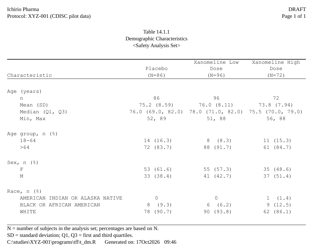
Demographic characteristics
From an ARD with a plan; the (N=xx) comes from the same
ARD. Explained step by step in Get
started.
Show code
ard_dm <- ard_stack(
  adsl, .by = TRT01A,
  ard_summary(variables = AGE,
              statistic = ~ continuous_summary_fns(
                c("N", "mean", "sd", "median", "p25", "p75", "min", "max"))),
  ard_tabulate(variables = c(AGEGR1, SEX, RACE)))

p_dm <- ard_dm |>
  normalize_ard() |>
  table_plan(cols = "TRT01A", rows = c(group = "variable")) |>
  plan_cells(
    continuous  = c("n"               = "{N:.0f}",
                    "Mean (SD)"       = "{mean:.1f} ({sd:.2f})",
                    "Median (Q1, Q3)" = "{median:.1f} ({p25:.1f}, {p75:.1f})",
                    "Min, Max"        = "{min:.0f}, {max:.0f}"),
    categorical = c(n == 0 ~ "0", "{n:.0f} ({p:.1f%})"),
    notes = FALSE) |>
  plan_labels(c(AGE = "Age (years)", AGEGR1 = "Age group, n (%)",
                SEX = "Sex, n (%)",  RACE   = "Race, n (%)")) |>
  plan_levels(AGEGR1 = c("18-64", ">64"), SEX = c("F", "M")) |>
  plan_stub(name = "row_label") |>
  plan_blanks(where = "between_groups", first = TRUE) |>
  plan_columns(widths = c(4, 2, 2, 2)) |>
  plan_style(border = "tfl", align_count_pct = TRUE) |>
  plan_col_header(values = list(n = TRUE), rtf_col_header(
    c("",               "{col}"),
    c("Characteristic", "(N={n})")))

doc <- rtf_document(
  page    = rtf_page(orientation = "portrait"),
  program = "/studies/XYZ-001/programs/tfl/t_dm.R",
  tokens  = list(STUDY = "XYZ-001")) |>
  rtf_section(
    header = rtf_header(list(
      c(l = "Ichirio Pharma",                      r = "DRAFT"),
      c(l = "Protocol: {STUDY} (CDISC pilot data)", r = "Page {PAGE} of {TOTAL_PAGES}"),
      c(c = ""),
      c(c = "Table 14.1.1"),
      c(c = "Demographic Characteristics"),
      c(c = "<Safety Analysis Set>"))),
    footer = rtf_footer(list(
      c(l = "N = number of subjects in the analysis set; percentages are based on N."),
      c(l = "SD = standard deviation; Q1, Q3 = first and third quartiles."),
      c(l = "{PROGRAM_FULL}    Generated on: {DATETIME}")))) |>
  rtf_tables(p_dm)
generate_rtfreport(doc, "t_dm.rtf", overwrite = TRUE)
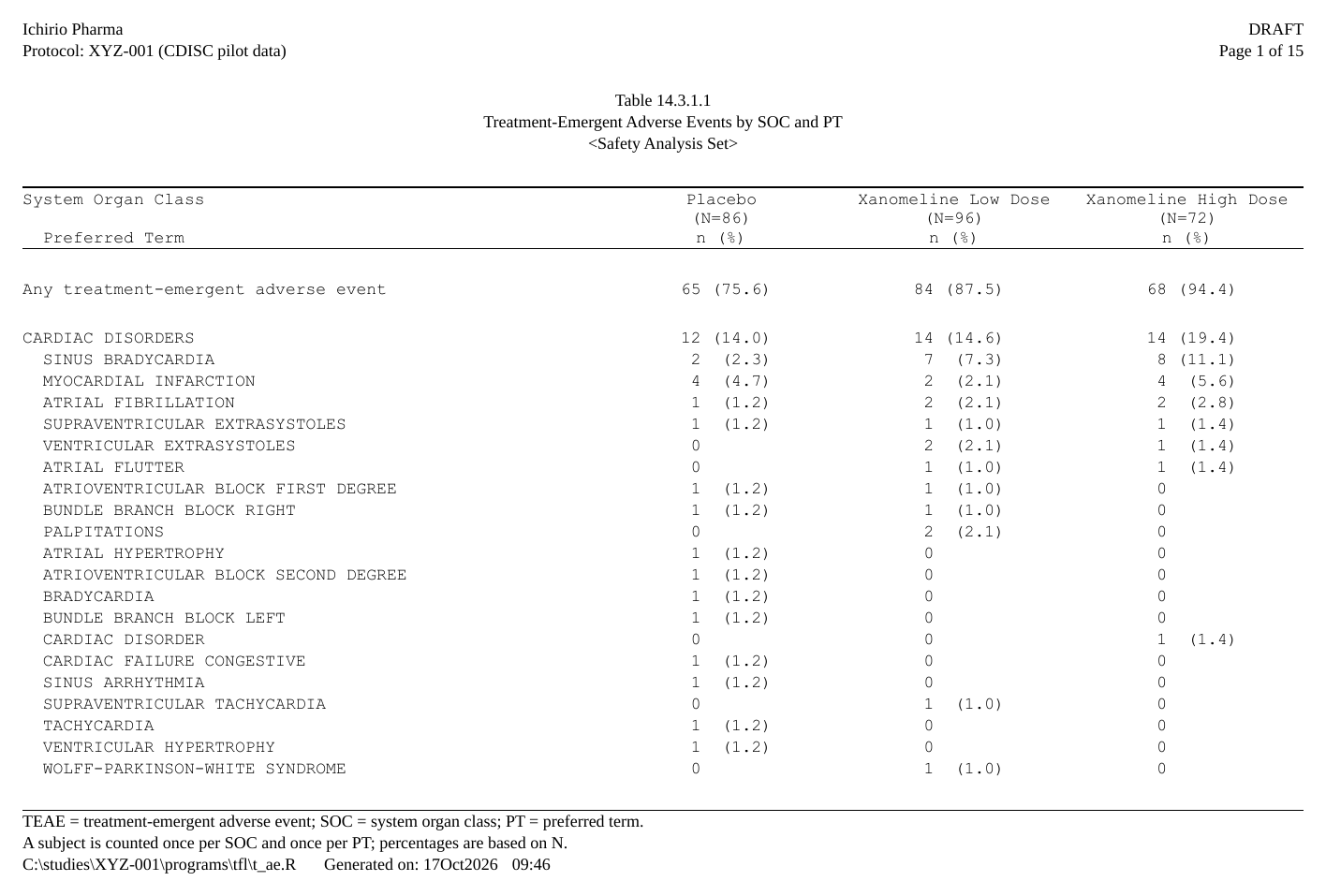
Adverse events by system organ class and preferred term
A hierarchical ARD sorted by frequency within each SOC, pages broken between SOCs. See Tables from an ARD.
Show code
adae <- pharmaverseadam::adae
adae <- adae[adae$TRTEMFL %in% "Y" & adae$SAFFL %in% "Y", ]
adae$TRT01A <- factor(adae$TRT01A, levels = arms)

ard_ae <- ard_stack_hierarchical(
  adae, variables = c(AEBODSYS, AEDECOD), by = TRT01A,
  denominator = adsl, id = USUBJID, over_variables = TRUE)

p_ae <- ard_ae |>
  normalize_ard(hierarchy = c("AEBODSYS", "AEDECOD"),
                overall = "Any treatment-emergent adverse event") |>
  table_plan(cols = "TRT01A", rows = c(SOC = "AEBODSYS", PT = "AEDECOD"),
             label = NA) |>
  plan_sort(".overall", "SOC", ".depth", "-n", "PT") |>
  plan_cells("{n:.0f} ({p:.1f%})", notes = FALSE) |>
  plan_stub(name = "System Organ Class\n  Preferred Term", indent = 2) |>
  plan_blanks(where = "between_groups", first = TRUE, counted = TRUE) |>
  plan_paginate_rows(max_rows = 25, split = "group_safe") |>
  plan_columns(widths = c(5, 2, 2, 2)) |>
  plan_style(border = "tfl", align_count_pct = TRUE) |>
  plan_col_header(values = list(n = TRUE), rtf_col_header(
    c("System Organ Class", "{col}"),
    c("  Preferred Term", "(N={n})\nn (%)")))

doc <- rtf_document(
  program = "/studies/XYZ-001/programs/tfl/t_ae.R",
  tokens  = list(STUDY = "XYZ-001")) |>
  rtf_section(
    header = rtf_header(list(
      c(l = "Ichirio Pharma",                      r = "DRAFT"),
      c(l = "Protocol: {STUDY} (CDISC pilot data)", r = "Page {PAGE} of {TOTAL_PAGES}"),
      c(c = ""),
      c(c = "Table 14.3.1.1"),
      c(c = "Treatment-Emergent Adverse Events by SOC and PT"),
      c(c = "<Safety Analysis Set>"))),
    footer = rtf_footer(list(
      c(l = "TEAE = treatment-emergent adverse event; SOC = system organ class; PT = preferred term."),
      c(l = "A subject is counted once per SOC and once per PT; percentages are based on N."),
      c(l = "{PROGRAM_FULL}    Generated on: {DATETIME}")))) |>
  rtf_tables(p_ae)
generate_rtfreport(doc, "t_ae.rtf", overwrite = TRUE)
length(plan_apply(p_ae))    # pages
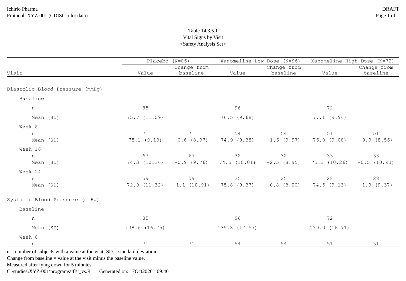
#> [1] 15Vital signs by visit
The value and the change from baseline under each arm, with a nested stub. See The plan verbs.
Show code
visits <- c("Baseline", "Week 8", "Week 16", "Week 24")
advs <- pharmaverseadam::advs
advs <- advs[advs$PARAMCD %in% c("SYSBP", "DIABP") &
               advs$ATPT %in% "AFTER LYING DOWN FOR 5 MINUTES" &
               (advs$ABLFL %in% "Y" | advs$ANL01FL %in% "Y") &
               advs$AVISIT %in% visits & advs$USUBJID %in% adsl$USUBJID, ]
advs$TRTA   <- factor(advs$TRT01A, levels = arms)
advs$AVISIT <- factor(advs$AVISIT, levels = visits)

stats <- ~ continuous_summary_fns(c("N", "mean", "sd"))
ard_vs <- bind_ard(
  ard_summary(advs, by = c(PARAM, AVISIT, TRTA), variables = AVAL,
              statistic = stats),
  ard_summary(droplevels(advs[advs$AVISIT != "Baseline", ]),
              by = c(PARAM, AVISIT, TRTA), variables = CHG,
              statistic = stats))

p_vs <- ard_vs |>
  normalize_ard() |>
  table_plan(cols = c("TRTA", "variable"),
             rows = c(PARAM = "PARAM", Visit = "AVISIT")) |>
  plan_levels(variable = c("AVAL", "CHG")) |>
  plan_cells(continuous = c("n"         = "{N:.0f}",
                            "Mean (SD)" = "{mean:.1f} ({sd:.2f})"),
             na = "", notes = FALSE) |>
  plan_stub(name = "Visit") |>
  plan_blanks(where = "between_groups", first = TRUE, last = TRUE) |>
  plan_columns(widths = c(5, rep(2, 6))) |>
  plan_style(border = "tfl") |>
  plan_col_header(values = list(n = c(table(adsl$TRT01A))), rtf_col_header(
    c(list(col_cell(1, "")),
      lapply(1:3, function(i) col_cell(c(2 * i, 2 * i + 1), "{col1} (N={n})"))),
    c("Visit", rep(c("Value", "Change from\nbaseline"), 3))))

doc <- rtf_document(
  program = "/studies/XYZ-001/programs/tfl/t_vs.R",
  tokens  = list(STUDY = "XYZ-001")) |>
  rtf_section(
    header = rtf_header(list(
      c(l = "Ichirio Pharma",                      r = "DRAFT"),
      c(l = "Protocol: {STUDY} (CDISC pilot data)", r = "Page {PAGE} of {TOTAL_PAGES}"),
      c(c = ""),
      c(c = "Table 14.3.5.1"),
      c(c = "Vital Signs by Visit"),
      c(c = "<Safety Analysis Set>"))),
    footer = rtf_footer(list(
      c(l = "n = number of subjects with a value at the visit; SD = standard deviation."),
      c(l = "Change from baseline = value at the visit minus the baseline value."),
      c(l = "Measured after lying down for 5 minutes."),
      c(l = "{PROGRAM_FULL}    Generated on: {DATETIME}")))) |>
  rtf_tables(p_vs)
generate_rtfreport(doc, "t_vs.rtf", overwrite = TRUE)
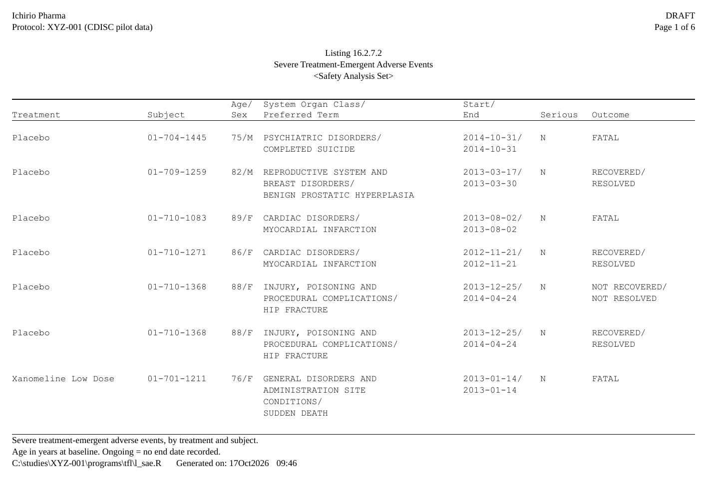
Listing of severe adverse events
Records, not statistics: cells wrap, keys print once, a record never splits. See Listings with a plan.
Show code
sae <- adae[adae$AESEV %in% "SEVERE", ]
sae <- merge(sae, adsl[, c("USUBJID", "AGE", "SEX")], by = "USUBJID",
             suffixes = c("", ".adsl"))
sae <- sae[order(sae$TRT01A, sae$USUBJID, sae$ASTDT), ]
sae$ASTDT <- format(sae$ASTDT, "%Y-%m-%d")
sae$AENDT <- ifelse(is.na(sae$AENDT), "Ongoing", format(sae$AENDT, "%Y-%m-%d"))

p_sae <- table_plan(sae) |>
  plan_listing(
    listing_col("TRT01A", width = 20, label = "Treatment", collapse_repeats = TRUE),
    listing_col("USUBJID", width = 12, label = "Subject", collapse_repeats = TRUE),
    listing_col(c("AGE", "SEX"), label = "Age/\nSex", layout = "flow"),
    listing_col(c("AEBODSYS", "AEDECOD"), width = 30,
                label = "System Organ Class/\nPreferred Term"),
    listing_col(c("ASTDT", "AENDT"), width = 11, label = "Start/\nEnd"),
    listing_col("AESER", label = "Serious"),
    listing_col("AEOUT", width = 16, label = "Outcome")) |>
  plan_blanks(where = "records") |>
  plan_paginate_rows(max_rows = 30) |>
  plan_style(border = "tfl")

doc <- rtf_document(
  program = "/studies/XYZ-001/programs/tfl/l_sae.R",
  tokens  = list(STUDY = "XYZ-001")) |>
  rtf_section(
    header = rtf_header(list(
      c(l = "Ichirio Pharma",                      r = "DRAFT"),
      c(l = "Protocol: {STUDY} (CDISC pilot data)", r = "Page {PAGE} of {TOTAL_PAGES}"),
      c(c = ""),
      c(c = "Listing 16.2.7.2"),
      c(c = "Severe Treatment-Emergent Adverse Events"),
      c(c = "<Safety Analysis Set>"))),
    footer = rtf_footer(list(
      c(l = "Severe treatment-emergent adverse events, by treatment and subject."),
      c(l = "Age in years at baseline. Ongoing = no end date recorded."),
      c(l = "{PROGRAM_FULL}    Generated on: {DATETIME}")))) |>
  rtf_tables(p_sae)
generate_rtfreport(doc, "l_sae.rtf", overwrite = TRUE)
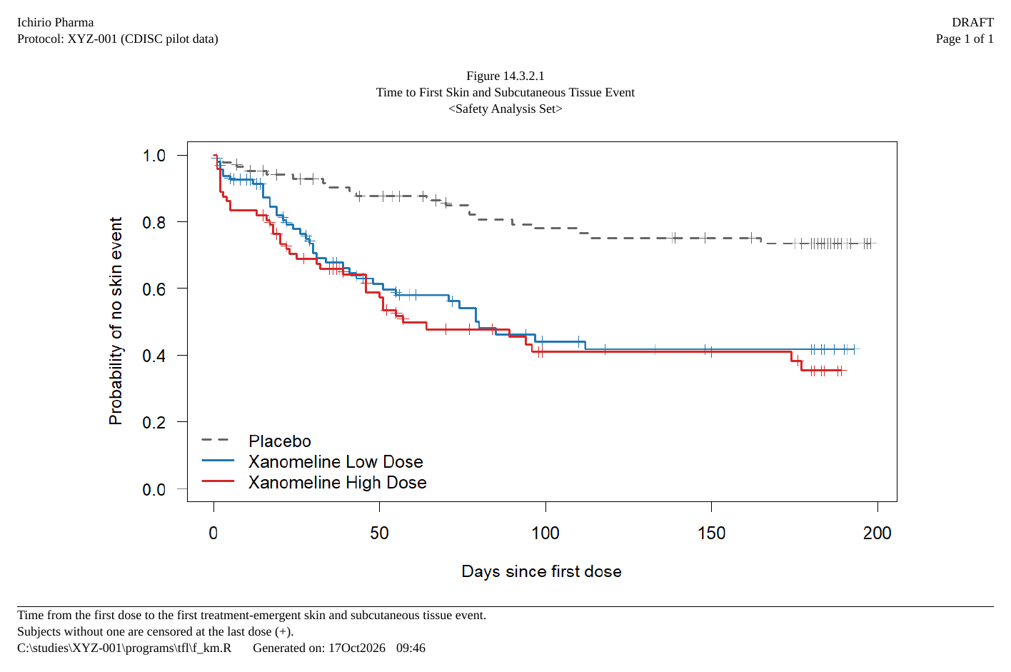
Kaplan-Meier plot
A figure is a page like any other, here drawn with base R and survival. See Figures.
Show code
# Time to the first treatment-emergent skin event, censored at the last dose
skin <- adae[adae$AEBODSYS %in% "SKIN AND SUBCUTANEOUS TISSUE DISORDERS", ]
first <- tapply(skin$ASTDT, skin$USUBJID, min)
tte <- adsl[!is.na(adsl$TRTEDT), c("USUBJID", "TRT01A", "TRTSDT", "TRTEDT")]
tte$event <- as.integer(tte$USUBJID %in% names(first))
tte$end   <- tte$TRTEDT
tte$end[tte$event == 1] <- as.Date(first[tte$USUBJID[tte$event == 1]])
tte$days  <- as.numeric(tte$end - tte$TRTSDT) + 1
fit <- survival::survfit(survival::Surv(days, event) ~ TRT01A, data = tte)

km <- function() {
  op <- par(mar = c(4.5, 4.5, 1, 1))
  on.exit(par(op))
  plot(fit, col = c("grey40", "#1f77b4", "#d62728"), lty = c(2, 1, 1),
       lwd = 2, mark.time = TRUE, xlab = "Days since first dose",
       ylab = "Probability of no skin event", las = 1)
  legend("bottomleft", legend = arms, col = c("grey40", "#1f77b4", "#d62728"),
         lty = c(2, 1, 1), lwd = 2, bty = "n")
}

doc <- rtf_document(
  program = "/studies/XYZ-001/programs/tfl/f_km.R",
  tokens  = list(STUDY = "XYZ-001")) |>
  rtf_section(
    header = rtf_header(list(
      c(l = "Ichirio Pharma",                      r = "DRAFT"),
      c(l = "Protocol: {STUDY} (CDISC pilot data)", r = "Page {PAGE} of {TOTAL_PAGES}"),
      c(c = ""),
      c(c = "Figure 14.3.2.1"),
      c(c = "Time to First Skin and Subcutaneous Tissue Event"),
      c(c = "<Safety Analysis Set>"))),
    footer = rtf_footer(list(
      c(l = "Time from the first dose to the first treatment-emergent skin and subcutaneous tissue event."),
      c(l = "Subjects without one are censored at the last dose (+)."),
      c(l = "{PROGRAM_FULL}    Generated on: {DATETIME}")))) |>
  rtf_figures(rtfplot(km, render_width = 8, render_height = 4.6,
                      render_dpi = 150))
generate_rtfreport(doc, "f_km.rtf", overwrite = TRUE)
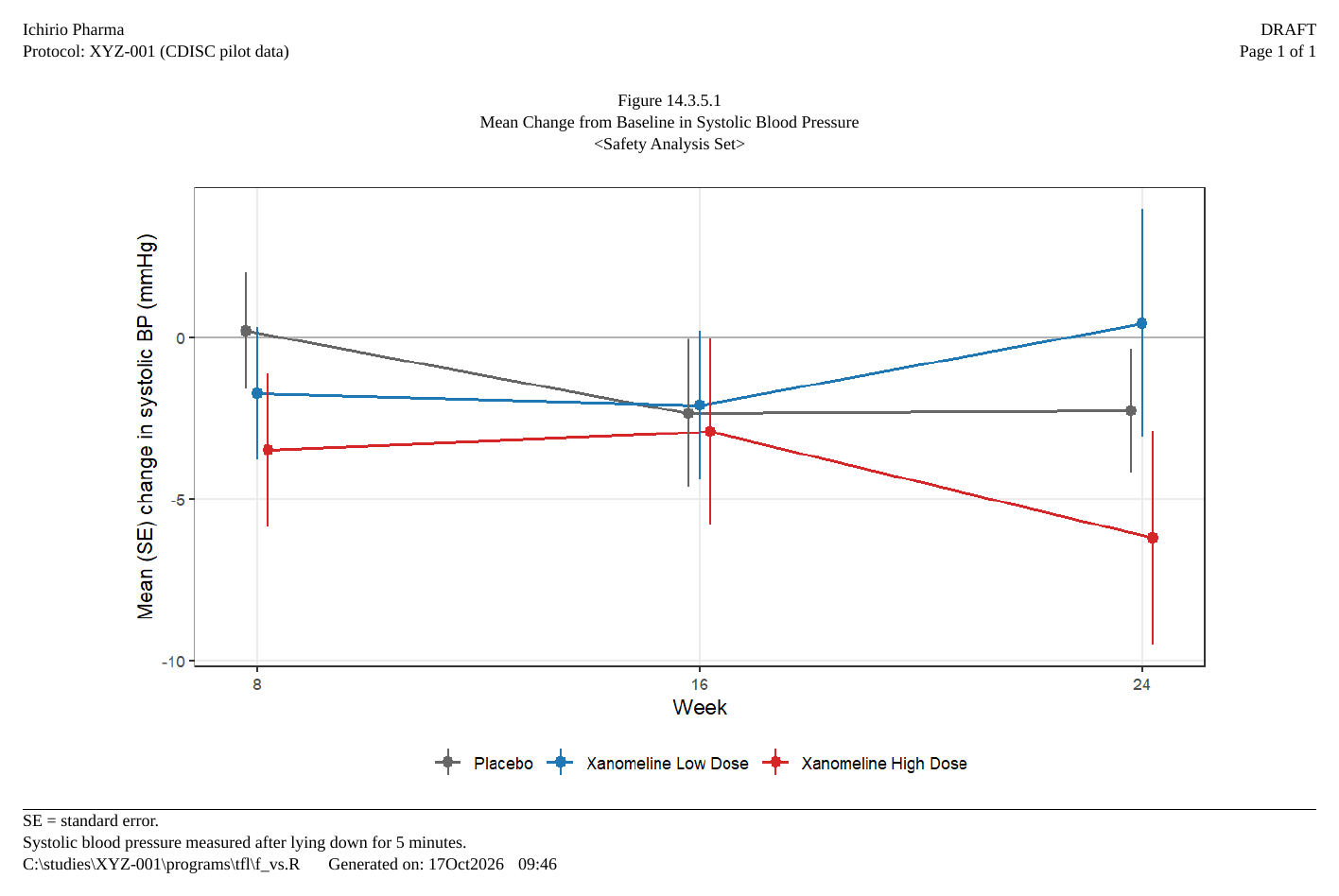
Mean change from baseline over time
A ggplot2 figure on the same page layout. See Figures.
Show code
library(ggplot2)

sbp <- advs[advs$PARAMCD == "SYSBP" & advs$AVISIT != "Baseline", ]
mc  <- aggregate(CHG ~ TRTA + AVISIT, data = sbp,
                 FUN = function(x) c(m = mean(x), se = sd(x) / sqrt(length(x))))
mc  <- do.call(data.frame, mc)
mc$week <- as.numeric(sub("Week ", "", mc$AVISIT))

g <- ggplot(mc, aes(week, CHG.m, colour = TRTA)) +
  geom_hline(yintercept = 0, colour = "grey70") +
  geom_line(linewidth = 0.7, position = position_dodge(0.6)) +
  geom_pointrange(aes(ymin = CHG.m - CHG.se, ymax = CHG.m + CHG.se),
                  position = position_dodge(0.6)) +
  scale_colour_manual(values = c("grey40", "#1f77b4", "#d62728")) +
  scale_x_continuous(breaks = c(8, 16, 24)) +
  labs(x = "Week", y = "Mean (SE) change in systolic BP (mmHg)", colour = NULL) +
  theme_bw(base_size = 11) +
  theme(legend.position = "bottom", panel.grid.minor = element_blank())

doc <- rtf_document(
  program = "/studies/XYZ-001/programs/tfl/f_vs.R",
  tokens  = list(STUDY = "XYZ-001")) |>
  rtf_section(
    header = rtf_header(list(
      c(l = "Ichirio Pharma",                      r = "DRAFT"),
      c(l = "Protocol: {STUDY} (CDISC pilot data)", r = "Page {PAGE} of {TOTAL_PAGES}"),
      c(c = ""),
      c(c = "Figure 14.3.5.1"),
      c(c = "Mean Change from Baseline in Systolic Blood Pressure"),
      c(c = "<Safety Analysis Set>"))),
    footer = rtf_footer(list(
      c(l = "SE = standard error."),
      c(l = "Systolic blood pressure measured after lying down for 5 minutes."),
      c(l = "{PROGRAM_FULL}    Generated on: {DATETIME}")))) |>
  rtf_figures(rtfplot(g, render_width = 8, render_height = 4.6,
                      render_dpi = 150))
generate_rtfreport(doc, "f_vs.rtf", overwrite = TRUE)
Where next
- Get started walks through the first table above step by step, and Tables from an ARD the others from an ARD.
- The plan verbs, Listings with a plan and Figures explain the pieces used here.
- Rendering, post-processing and assembly joins finished files like these into one deliverable with a table of contents.