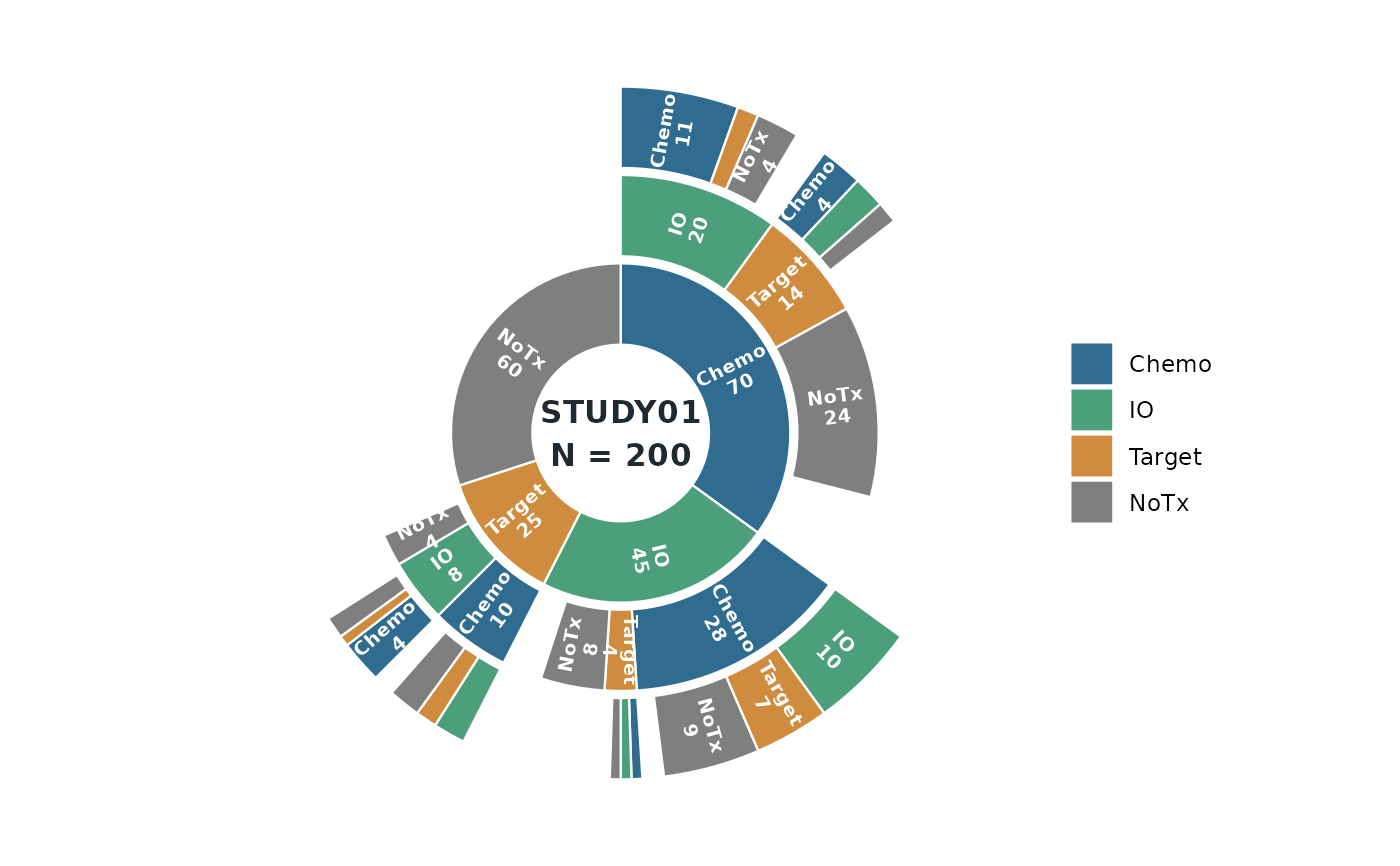
Plot a Static Sunburst of Treatment Sequences — tfl_plot

Draw a treatment-pattern sunburst (ring chart) using ggplot2 primitives only (geom_rect + coord_polar + geom_text) – the output is a fully static ggplot object suitable for publications and regulatory documents.

Usage

tfl_plot_sunburst(
  paths,
  path_cols = NULL,
  path_value = "n",
  levels = NULL,
  segment_labels = NULL,
  palette = NULL,
  segment_color = "white",
  ring_height = 0.92,
  inner_radius = 1,
  show_labels = TRUE,
  label_size = 2.6,
  label_color = "white",
  label_min_frac = 0.02,
  center_label = NULL,
  center_size = 4.2,
  center_color = "#1F2A30"
)

Arguments

paths: A data frame of treatment sequences (one row per path).
path_cols: Character vector naming the ring columns of paths, in ring order (inner first). Default: every column except path_value, in the order they appear.
path_value: Column name in paths holding the patient count of each path.
levels: Optional character vector fixing the order of the segment categories within every ring. Default: order of first appearance across the ring columns.
segment_labels: Optional named character vector mapping a category to the display text used on the arcs and in the legend (e.g. c(IO = "Immunotherapy")). Unmapped categories show verbatim.
palette: Optional colour palette for the categories. A named vector is matched by category name; an unnamed vector is recycled over levels. Default: grDevices::hcl.colors() "Set 2".
segment_color: Border colour of the arcs.
ring_height: Radial thickness of each ring, in (0, 1] ring units.
inner_radius: Radius of the centre hole, in ring units.
show_labels: Whether to draw the arc labels.
label_size: Arc label size.
label_color: Arc label colour.
label_min_frac: Minimum share of the full circle an arc must span for its label to be drawn (labels on thinner arcs are suppressed).
center_label: Optional text drawn in the centre hole (e.g. "STUDY01\nN = 200").
center_size: Centre label size.
center_color: Centre label colour.

Value

A ggplot object.

Details

Each ring is one treatment line (the innermost ring is the first line) and the arc length is the number of patients (one patient = one angular unit, so no normalisation is applied). The child arcs of a segment start at the parent's start angle and nest inside the parent's span; whatever remains of the parent's span stays empty – those are the patients with no further treatment line (attrition), the same idea as the unlinked part of a tfl_plot_sankey() node.

The input is a path table: one row per treatment sequence, with one column per ring (path_cols) and a count column (path_value). NA (or "") in a ring column means the path stops before that ring; once a path has stopped it must stay NA in all later columns. Rows describing the same sequence are summed.

Examples

# One shared dataset, two views. This path table is the first three lines
# of the tfl_plot_sankey() example's 200-patient cohort: one row per treatment
# sequence (C = Chemo, IO = Immunotherapy, T = Targeted, N = No
# Treatment), `n` patients per path (L1 200 -> L2 120 -> L3 70, about 30%
# "No Treatment" per line, no same-treatment transitions). A name like
# "C,IO" is a path that stops after the second line.
seq_n <- c(
  "C,IO,C" = 11, "C,IO,T" = 2, "C,IO,N" = 4, "C,IO" = 3,
  "C,T,C" = 4, "C,T,IO" = 3, "C,T,N" = 2, "C,T" = 5,
  "C,N" = 24, "C" = 12,
  "IO,C,IO" = 10, "IO,C,T" = 7, "IO,C,N" = 9, "IO,C" = 2,
  "IO,T,C" = 1, "IO,T,IO" = 1, "IO,T,N" = 1, "IO,T" = 1,
  "IO,N" = 8, "IO" = 5,
  "T,C,IO" = 3, "T,C,T" = 2, "T,C,N" = 3, "T,C" = 2,
  "T,IO,C" = 4, "T,IO,T" = 1, "T,IO,N" = 2, "T,IO" = 1,
  "T,N" = 4, "T" = 3,
  "N" = 60
)
parts <- strsplit(names(seq_n), ",")
paths <- data.frame(
  line1 = vapply(parts, `[`, character(1), 1),
  line2 = vapply(parts, `[`, character(1), 2),
  line3 = vapply(parts, `[`, character(1), 3),
  n = unname(seq_n),
  stringsAsFactors = FALSE
)

trt <- c(C = "Chemo", IO = "Immunotherapy", T = "Targeted",
         N = "No Treatment")
trt_colors <- c(C = "#2F6C8F", IO = "#4B9F7A", T = "#D08C3E",
                N = "#7F7F7F")

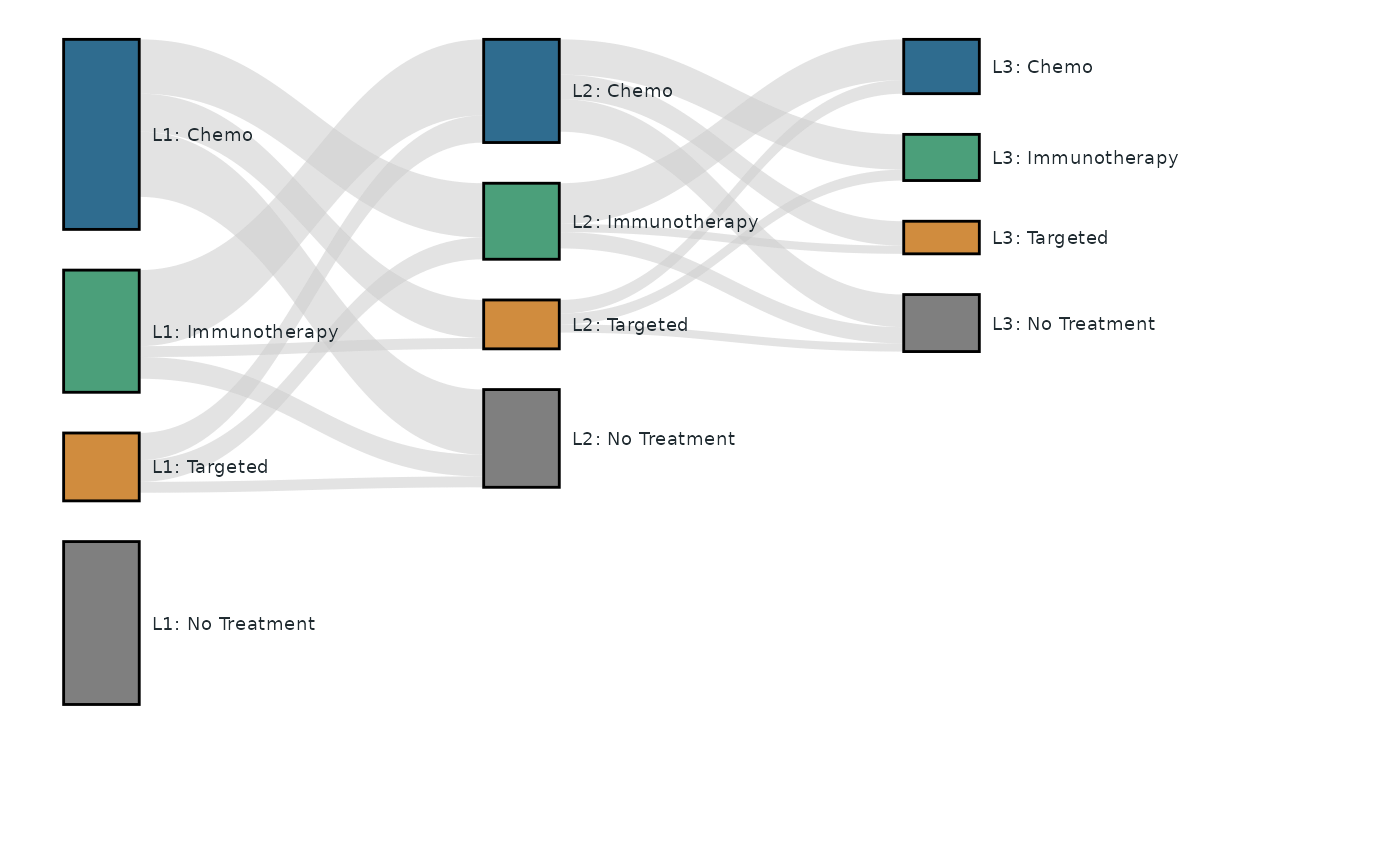
# The SAME paths feed a sankey: per-line totals give the node sizes
# (including the link-less "L1: No Treatment" node) and consecutive-line
# transitions give the links -- exactly the L1-L3 slice of the
# tfl_plot_sankey() example's node and link tables.
ring <- c("line1", "line2", "line3")
nodes <- do.call(rbind, lapply(1:3, function(k) {
  data.frame(
    id        = paste0("L", k, "_", names(trt)),
    stage     = paste0("Line", k),
    line      = paste0("Line", k),
    treatment = unname(trt),
    label     = paste0("L", k, ": ", unname(trt)),
    node_n    = as.vector(tapply(paths$n, paths[[ring[k]]], sum)[names(trt)]),
    stringsAsFactors = FALSE
  )
}))
links <- do.call(rbind, lapply(1:2, function(k) {
  move <- !is.na(paths[[ring[k + 1]]])
  agg <- aggregate(
    list(value = paths$n[move]),
    list(s = paths[[ring[k]]][move], t = paths[[ring[k + 1]]][move]),
    sum
  )
  data.frame(
    source = paste0("L", k, "_", agg$s),
    target = paste0("L", k + 1, "_", agg$t),
    value  = agg$value,
    stringsAsFactors = FALSE
  )
}))

# Transition view: who moves where between lines.
tfl_plot_sankey(
  nodes = nodes,
  links = links,
  node_id = "id",
  node_stage = "stage",
  node_label = "label",
  node_value = "node_n",
  link_source = "source",
  link_target = "target",
  link_value = "value",
  node_treatment = "treatment",
  node_line = "line",
  treatment_color_mode = "across_lines",
  treatment_palette = stats::setNames(trt_colors, trt),
  baseline = "top",
  link_alpha = 0.55,
  label_size = 2.5
)


# Path view of the very same data: each ring is a treatment line, arc
# length is patients, and the empty remainder of a parent arc is the
# attrition (the sunburst counterpart of the sankey's unlinked node span).
tfl_plot_sunburst(
  paths,
  path_cols = ring,
  path_value = "n",
  levels = names(trt),
  segment_labels = c(C = "Chemo", IO = "IO", T = "Target", N = "NoTx"),
  palette = trt_colors,
  center_label = "STUDY01\nN = 200"
)